During the optimisation process, we are trying to optimise two things: the ice itself and the behaviour of the protein within the ice.
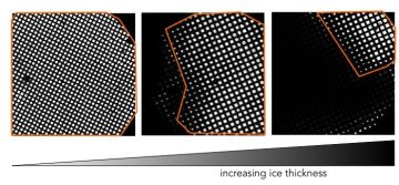
Grids can have different amounts of thick ice; usable areas highlighted in orange.
The first thing we look at is a low magnification montage of the entire grid. The ice thickness can vary across the grid, but we want to see bright squares because when the ice is extremely thick the beam will not be able to penetrate and you will not see the grid bars.
We will then look at individual grid squares at medium magnification. Within a square you will see a regular pattern of holes, which may or may not have ice within them. The contrast between the holes and the surrounding carbon is indicative of the ice thickness, which can vary within a grid square.
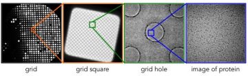
Increasing magnifications- from grid, to square, to grid holes, to protein
For the first screening, we will often try multiple freezing conditions rather than varying the protein conditions, as it is quite likely some of the freezing parameters will result in grids with too thick or too thin ice. We may be able to find few squares in which the ice has a good thickness but we will often want to increase the amount of these squares by optimising the ice. This is done by changing the freezing parameters, and sometimes will not be a trivial process. Ultimately, we are looking for grids that have enough ice in which the protein looks good to collect data from.
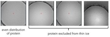
Protein can be excluded when ice is too thin
It is worth noting that sample behaviour can change depending on ice thickness: for some particles, when the ice is too thin the particle will be unable to enter and so we will see particles distributed unevenly. We want to find ice that is as thin as possible without affecting particle behaviour to maximise contrast between the particle and the surrounding ice. As the ice thickness will vary across the grid, we will try imaging in different regions to determine what thickness of ice to target.
The final step is to look in the holes themselves at a high magnification to see if we can visualise your sample. We may see a number of behaviours: no sample in the holes; too much sample in the holes; aggregation of protein; sample sticking to the carbon at the edge of the hole; sample evenly distributed in the holes. Do not be discouraged if the protein does not look good the first time! If we can see protein at all in the holes, this is a good sign as it gives a starting point for optimisation.
Issues we may encounter include:
-
Concentration
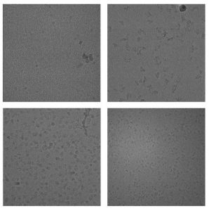
Protein should be dilute enough that particles can be easily distinguished, but concentrated enough that there are a good number of particles per image.
Concentration of the protein in the holes does not always scale linearly. Proteins may preferentially bind to the carbon support, and so the concentration in the holes may not increase until the carbon is saturated.
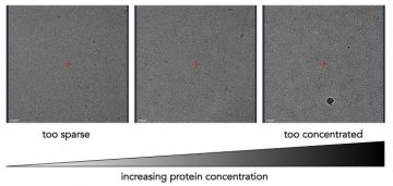
Examples of the same protein at different concentrations.
-
-Aggregation
Interaction with the air-water interface can cause proteins to denature and aggregate on the grid. Sometimes interaction with the carbon can also induce aggregation.
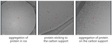
Protein can aggregate at the-air water interface, or on the carbon support.
-
Preferential Orientation
Some proteins will appear in a preferred orientation i.e. with only one view of the protein present. In order to reconstruct a 3D volume from 2D projection images we need multiple views of the protein.
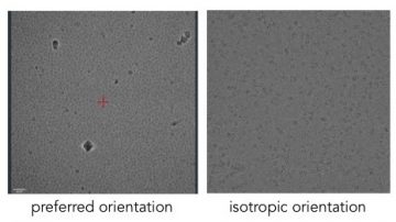
Proteins can adopt preferred orientations at the air-water interface.
Optimising every project is different and facility staff will consult with you to help! There is no one-size-fits-all solution and we will advise based on how your protein is behaving. Some techniques that we can use for optimization can include:
Examples of samples we have collected in at HRMEM.
- Addition of detergent
- Use of grids with support film
- Change in grid type (e.g. Quantifoil vs C-Flat, holey carbon vs. lacy)
- Change in protein buffer conditions
It is always worth keeping in mind that optimising the protein purification may help more than trying to improve a sub-optimal preparation through grid optimisation. For example, contaminants may preferentially enter the holes resulting in a false impression, or can even induce aggregation on the grid. Similarly, adding a binding partner or antibody may stabilise your protein of interest. For membrane proteins, the choice of membrane mimetic can dramatically alter how the protein behaves.
There is always a balance between continuing to optimise and deciding to collect data. Spending time optimising your grids can save time and money later on. However, you can spend a lot of time tweaking parameters and still ever achieve the ‘perfect’ sample. When the sample is of sufficient quality we will collect a small dataset to analyse. This can often tell us whether it is worth collecting a lot of data or if there needs to be more optimisation of the sample.